How it works¶

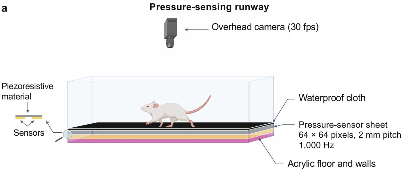
TactileArena measures contact directly. The floor operates as a pressure-imaging sensor, sampled fast enough to resolve load dynamics within individual steps and recorded on the same clock as overhead video.

Sensing surface¶

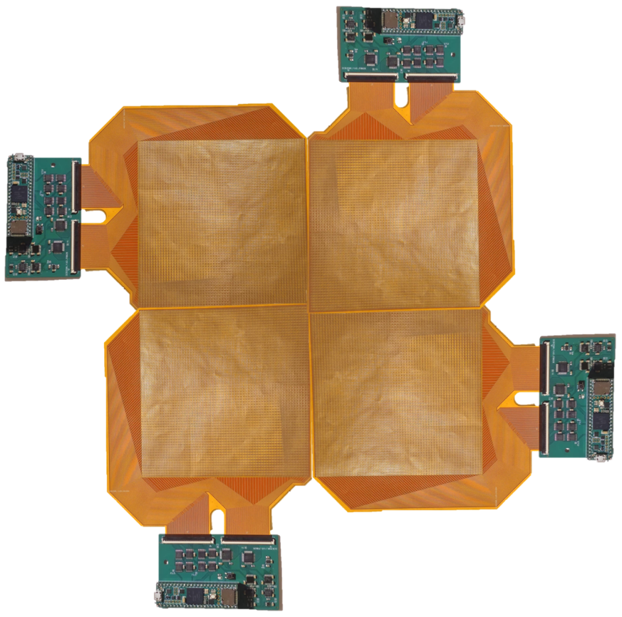
Each module is a flexible printed circuit carrying a 64 × 64 array of electrode pairs at 2-mm pitch: 4,096 tactile pixels (taxels) over 128 × 128 mm. A piezoresistive film covers the array, and applied pressure reduces its resistance between the underlying electrodes. A waterproof cloth covers the assembly, so that the animal does not contact the electronics.

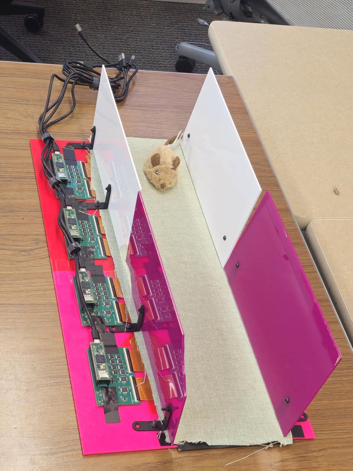
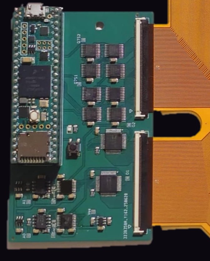
Each module is read by a dedicated readout board (a Teensy 4.1 microcontroller with analog multiplexers and analog-to-digital converters) connected directly to the module's flexible tails. Four modules placed side by side form the 64 × 256-taxel runway: 16,384 taxels over 512 × 128 mm, enclosed by transparent walls beneath an overhead camera.

Because each module is read independently, the modules can be arranged in other geometries, such as a square open-field arena (Modularity; Supplementary Video 5 on the Paper page).

Schematic of the runway: overhead camera, transparent walls, waterproof cloth over the pressure-sensor sheet and piezoresistive layer, acrylic floor. — **Runway configuration.** An overhead camera above the pressure-sensor sheet and piezoresistive layer, covered by a waterproof cloth and enclosed by transparent walls.

The assembled runway: an acrylic base with four readout boards along one side, acrylic walls and a cloth-covered sensing floor. — Assembled runway: four modules beneath the cloth between the walls, with the four readout boards along one side (a toy mouse is shown for scale).

A readout board: Teensy 4.1, eight shift registers, two multiplexers, two analog-to-digital converters and two flexible-circuit connectors holding the sensor tails. — Readout board: a Teensy 4.1, shift registers that drive the rows, multiplexers and analog-to-digital converters that read the columns, and two connectors for the sensor tails.

Four sensor modules tiled two by two with their four readout boards. — Four modules tiled in a 2 × 2 configuration.

Adaptive compressive sampling¶

In a conventional raster-scanned pressure array, every taxel is measured in each frame, so that increasing the sensing area or density reduces the frame rate. During locomotion, however, only a small fraction of the surface is loaded at any moment. The readout firmware therefore concentrates its measurements on active contacts (adaptive compressive sampling; Slepyan et al., 2024).

In each frame, every board measures a fixed budget of M taxels (M = 200, 4.9% of the module, in the study recordings) in the following order:

Tracking of active contacts. Taxels that triggered neighbourhood sampling in the previous frame are measured first.
Background scan. The remaining budget follows a fixed coarse-to-fine pattern that begins at the module centre and continues through grids of successively halved pitch (32, 16, 8, 4 and 2 taxels), so that an incomplete scan still covers the module uniformly. The pattern shifts by one column each frame, and by one row after each full sweep of columns, so that every taxel is measured across successive frames.
Neighbourhood expansion. Whenever a reading exceeds the threshold T, the unmeasured taxels in its 3 × 3 neighbourhood are measured, recursively, so that each contact is captured at full resolution together with a boundary of unloaded taxels.

Each taxel is measured at most once per frame, and all measurements, including those below threshold, are transmitted to the host computer. In the study recordings (M = 200, T = 700 ADC counts), each board produced a frame approximately every millisecond.

Interactive simulation¶

The left panel shows the pressure applied to one module by a simulated paw that follows the pointer (press and drag; in the absence of input, two simulated paws traverse the module). The right panel shows the taxels measured by the firmware's sampling loop in the current frame.

Reducing M makes the background scan sparser while contacts remain fully resolved; increasing T restricts neighbourhood expansion to more strongly loaded regions. The simulation is displayed at approximately 30 frames per second; the readout boards operate at approximately 1,000.

Recorded acquisition frames¶

The display below reproduces the recorded data: for each of the four boards, the taxels measured in its most recent frame during 0.6 s of walking (rat 4, 24 February 2026, before surgery).

Modules without active contacts allocate their full budget to the background scan, which therefore reaches a finer grid level in those modules.

Configurable acquisition¶

M and T are transmitted to each board at the start of a recording, so that the balance between frame rate and background coverage is set in software. A smaller M yields a higher frame rate with sparser background coverage per frame, and a larger M the converse. The threshold defines the minimum load treated as contact, and a programmable amplifier gain (digital potentiometer) sets sensitivity for the expected loading range. The nominal 1-kHz frame rate is therefore a property of the configuration used in the study.

Force calibration¶

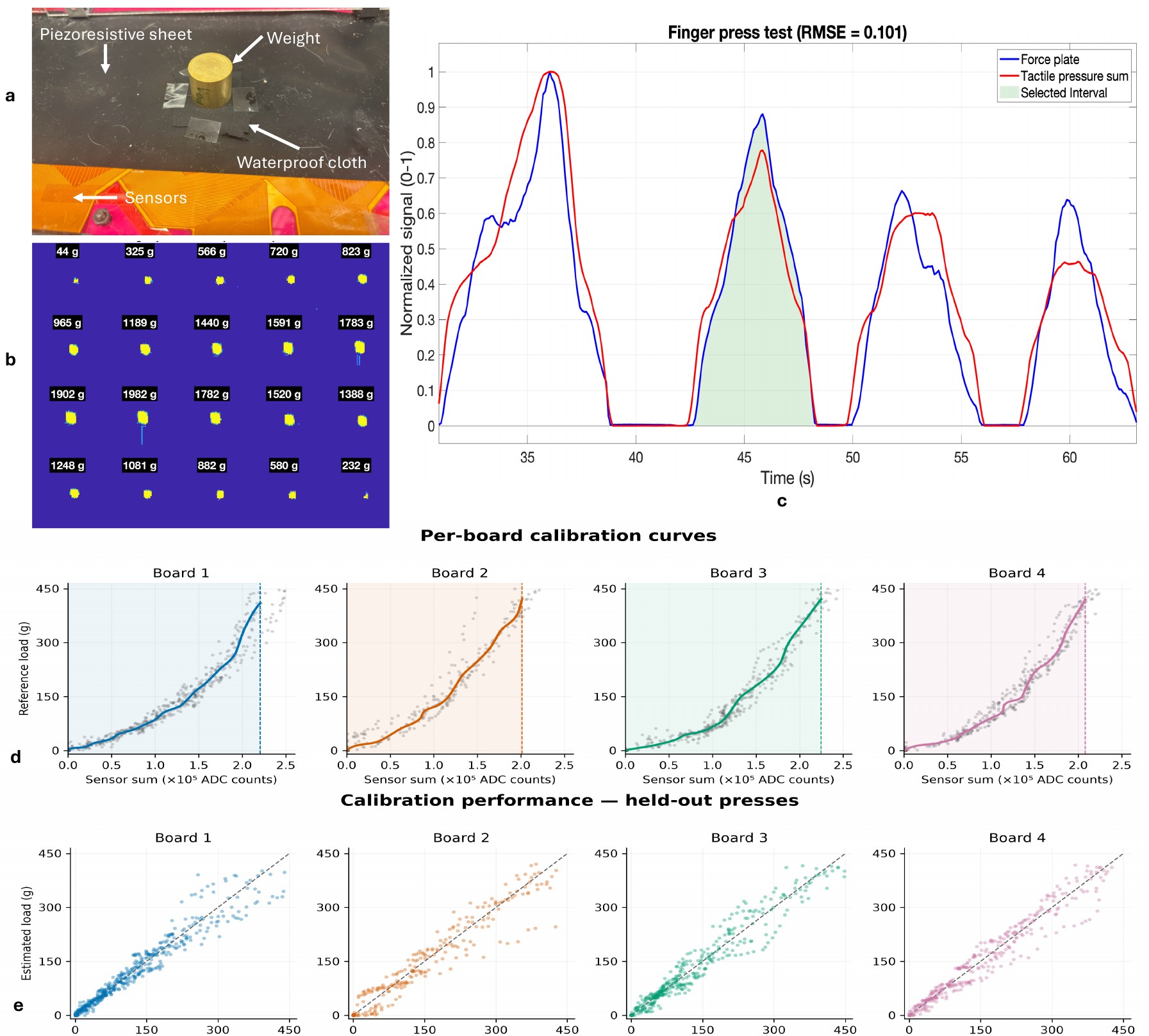
Raw taxel responses are converted to load using board-specific calibration curves. Each module was loaded through the same waterproof cover on an independent force plate (three load cells with a 24-bit amplifier). The summed tactile response followed the loading and unloading phases of the force-plate signal (RMSE 0.101 between independently normalized signals). Piecewise cubic Hermite curves, one per board, map summed responses to mass-equivalent load between 0 and approximately 410–421 g.

On presses withheld from the fit, the curves predicted load with RMSE of 23.4–30.6 g, approximately 5–8% of the body mass of the rats studied. The nerve-injury analyses normalize loading by body mass and compare each animal with its own presurgical baseline.

Calibration setup, pressure-map snapshots during a press, force-plate and tactile signals, per-board calibration curves and held-out-press performance. — **Characterization.** Tactile and force-plate responses, per-board calibration curves (d) and held-out-press predictions (e). Supplementary Fig. S1 of the manuscript.

Analysis pipeline¶

Pipeline: high-speed pressure frames and overhead video; a convolutional network localizes the tail base; registration fuses video and pressure; contacts are assigned to paws and linked into footsteps. — **Analysis pipeline** (Fig. 1 of the manuscript). A1, pressure frame as acquired; black taxels were not measured in that frame. A2, overhead video. B, tail-base localization. C, registered fusion. D, paw assignment. E, footstep extraction.

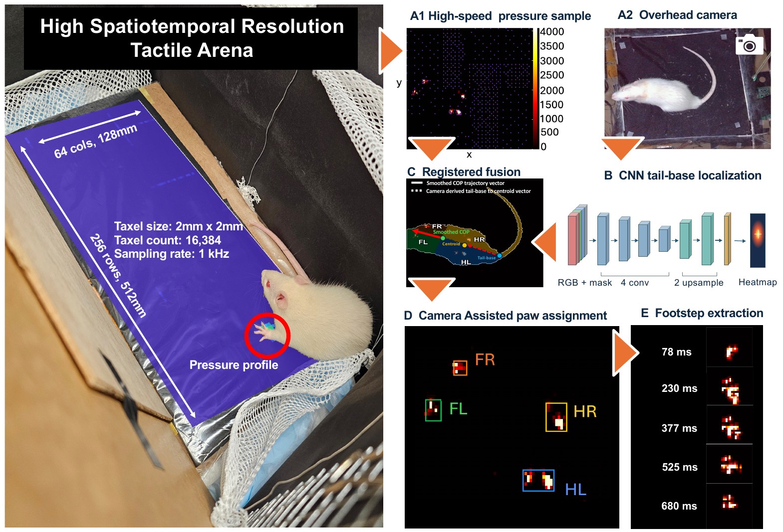
Synchronization. Pressure packets from the four boards and frames from the overhead and side cameras are timestamped against a common host clock from a shared start signal.
Pressure frames. The most recent packet from each board is reconstructed into a 64 × 64 image (taxels not measured in that frame were below threshold in recent frames and are set to zero), and the four images are combined into the 64 × 256 runway map.
Registration. A projective transform, defined from the platform corners in each recording, maps video frames onto the taxel grid; background subtraction yields the body mask.
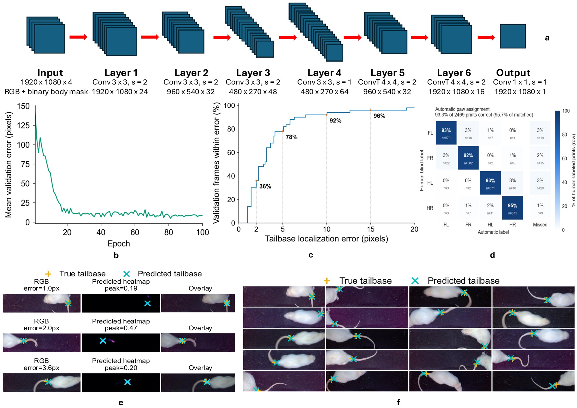
Body orientation. A convolutional encoder–decoder localizes the tail base from the image and body mask; the vector from the tail base to the body centroid defines body orientation.
Paw assignment. Pressure contacts are tracked across frames, segmented into stance events, and scored for each paw according to their position relative to the smoothed whole-animal centre of pressure and walking direction. Camera-derived votes contribute a weighted term, and Viterbi decoding enforces consistent left/right sequences.

Within manually curated walking windows from 81 recordings, the pipeline correctly identified 2,303 of 2,469 manually annotated contacts (93.3%; 95.7% of matched contacts). Walking windows are proposed automatically from the COP speed and curated manually, and camera-to-sensor registration uses manually identified platform corners.

Tail-base network architecture, training curves, localization accuracy, paw-assignment confusion matrix and examples. — **Tail-base localization and paw-assignment accuracy** (Supplementary Fig. S2). Panel d shows the confusion matrix for all 2,469 manually annotated contacts.

Measures computed for each contact¶

Measure	Definition
Stance, stride and duty factor	contact onset and lift-off of each paw; duty factor = stance duration / stride duration
Contact area and shape	area of the thresholded footprint (4 mm² per taxel) and length-to-width ratio
Peak and time-integrated load	summed response per contact, calibrated to mass-equivalent grams, and its integral over stance
Centre of pressure (COP)	pressure-weighted centroid for the whole animal or within an individual paw
Interlimb ratios and imbalance	left-to-right hindpaw duty-factor and loading ratios; (L−R)/(L+R) during hindpaw-only support

The Software page describes how to run the pipeline; all parameters are given in the Methods of the manuscript.

Limitations¶

The piezoresistive film measures normal pressure; tangential (shear) forces are not measured.
Calibration was performed per board on summed responses rather than per taxel; held-out errors were 23.4–30.6 g.
The 2-mm pitch resolves the plantar contact geometry of the rat paw; smaller animals would require finer-pitch sensors.
Automated paw assignment was validated within walking bouts; turning, overlapping contacts and prolonged spontaneous behaviour require further validation.